Distribution X Equals 0 Probability Is 0.0: A Deep Dive Into The World Of Zero Probability Distributions

Jovany Stanton DDS 24 May 2025

Have you ever wondered about the intricacies of probability distributions? Today, we’re diving deep into a fascinating concept: when distribution X equals 0, the probability is 0.0. This might sound like a mouthful, but trust me, it’s about to get interesting. Imagine a world where numbers don’t just represent values—they tell stories. In this article, we’ll explore the concept of zero probability distributions, breaking it down so even the most curious minds can understand.

Now, I know what you’re thinking. “Why does this matter?” Well, buckle up because this concept has real-world applications in fields like statistics, finance, and even quantum mechanics. Whether you’re a student trying to ace your math class or a professional looking to sharpen your analytical skills, understanding this idea is crucial. So, let’s get started!

Before we dive into the nitty-gritty, let’s clarify something. Zero probability distributions aren’t as scary as they sound. They’re simply a way to describe situations where certain outcomes are impossible. Think of it like rolling a six-sided die and expecting to roll a seven—it’s just not going to happen. Stick around, and by the end of this article, you’ll have a solid grasp of this concept.

What Exactly is a Distribution X Equals 0 Probability?

Let’s break it down. When we talk about a distribution where X equals 0 and the probability is 0.0, we’re essentially discussing a scenario where a specific outcome has absolutely no chance of occurring. This might seem straightforward, but the implications are profound.

For instance, consider a random variable X that represents the number of heads you get when flipping a coin. If X is defined as the number of heads in a single flip, the probability of getting two heads (X = 2) is 0. Why? Because it’s physically impossible to flip a coin once and get two heads. Simple, right?

Why Does Zero Probability Matter?

Zero probability matters because it helps us define the boundaries of what’s possible. In statistical models, understanding which outcomes are impossible allows us to create more accurate predictions. For example, in machine learning, algorithms can use this concept to filter out impossible scenarios, improving their overall performance.

It helps refine models by eliminating impossible outcomes.
It ensures that predictions are grounded in reality.
It provides a clear framework for understanding complex systems.

Key Characteristics of Zero Probability Distributions

Zero probability distributions have some unique characteristics that set them apart. Let’s take a closer look:

1. Impossible Outcomes

The most obvious characteristic is that they represent outcomes that cannot happen. This is often due to physical or logical constraints. For example, if X represents the number of planets in a solar system, the probability of X being negative is 0 because you can’t have a negative number of planets.

2. Discrete vs. Continuous Distributions

Zero probability can occur in both discrete and continuous distributions. In discrete distributions, it means certain values are impossible. In continuous distributions, it means the probability of any single exact value is 0. Think about it—what’s the chance of randomly picking the exact number 3.14159 from an infinite range of real numbers? Pretty slim, right?

Applications in Real Life

Now that we’ve covered the basics, let’s talk about how this concept applies to real-world situations. Zero probability distributions aren’t just theoretical—they have practical uses in various fields.

1. Finance

In finance, zero probability distributions help analysts assess risk. For example, if a stock price is modeled using a normal distribution, the probability of the price being negative is 0. This ensures that financial models remain realistic and reliable.

2. Engineering

Engineers use zero probability to design systems that operate within safe parameters. For instance, if a bridge’s load capacity is modeled using a probability distribution, the probability of exceeding the maximum safe load is 0. This guarantees the bridge’s structural integrity.

3. Medicine

In medical research, zero probability distributions help identify impossible outcomes in clinical trials. For example, if a drug is being tested for its effectiveness, the probability of a patient receiving both the drug and a placebo simultaneously is 0. This ensures the trial’s results are valid.

The Math Behind Zero Probability

Let’s dive into the math a bit. The concept of zero probability is rooted in probability theory. Here’s a quick breakdown:

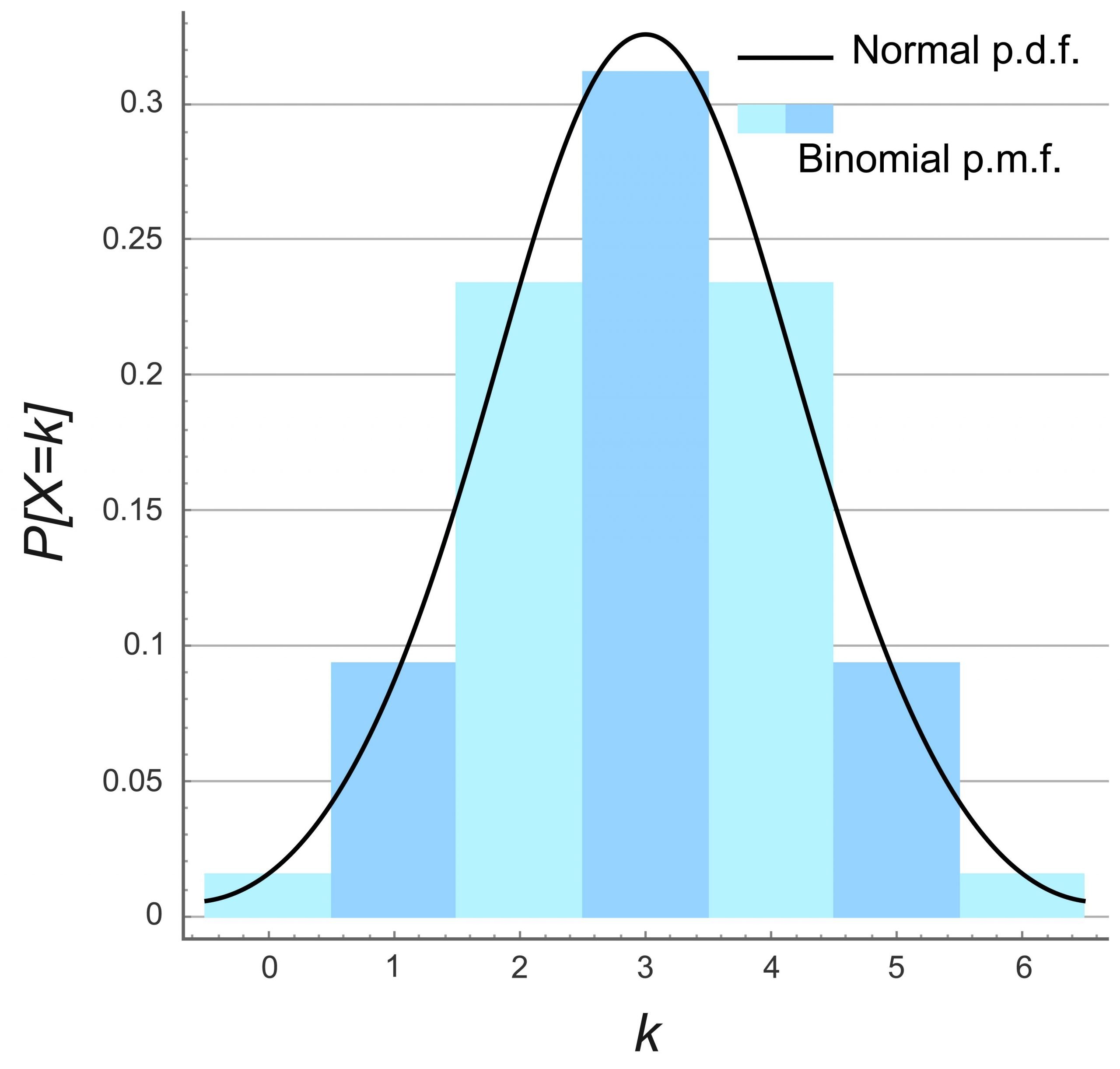
1. Probability Mass Function (PMF)

In discrete distributions, the PMF assigns probabilities to each possible value. If a value has a probability of 0, it means that value cannot occur. For example, if X represents the number of tails in a single coin flip, the PMF for X = 2 is 0.

2. Probability Density Function (PDF)

In continuous distributions, the PDF describes the likelihood of a random variable taking on a specific value. However, the probability of any single exact value in a continuous distribution is 0. Instead, we calculate probabilities over intervals.

Common Misconceptions

There are a few misconceptions about zero probability distributions that we need to clear up:

1. Zero Probability Means Impossible

Some people think that zero probability means an event is theoretically impossible. While this is true in many cases, it’s not always the case in continuous distributions. For example, the probability of randomly selecting an exact number from a continuous range is 0, but it doesn’t mean the event is impossible—it just means the likelihood is infinitesimally small.

2. Zero Probability Implies No Data

Another misconception is that zero probability means there’s no data to support a particular outcome. This isn’t necessarily true. In some cases, the data simply doesn’t support the occurrence of a specific value, but that doesn’t mean the data is incomplete.

How to Work with Zero Probability Distributions

Working with zero probability distributions requires a solid understanding of probability theory. Here are a few tips:

1. Define the Sample Space

Start by defining the sample space, which is the set of all possible outcomes. This will help you identify which outcomes have zero probability.

2. Use Appropriate Models

Choose the right probability model for your situation. Whether it’s a discrete or continuous distribution, make sure it accurately reflects the real-world scenario you’re analyzing.

3. Validate Your Results

Always validate your results against real-world data. If your model predicts zero probability for an event that actually occurs, it’s time to revisit your assumptions.

Case Studies

Let’s look at a couple of case studies to see how zero probability distributions are applied in practice:

1. Weather Forecasting

Weather forecasters use zero probability distributions to predict extreme weather events. For example, the probability of a hurricane forming in the Arctic Ocean is 0. This helps meteorologists focus their resources on more likely scenarios.

2. Sports Analytics

In sports analytics, zero probability distributions help teams identify impossible outcomes. For instance, the probability of a basketball player scoring 100 points in a single game is 0, but that doesn’t stop analysts from studying other factors that contribute to success.

Conclusion

So there you have it—a deep dive into the world of zero probability distributions. From understanding the basics to exploring real-world applications, we’ve covered a lot of ground. Here’s a quick recap:

Zero probability distributions describe outcomes that cannot occur.
They have applications in finance, engineering, medicine, and more.
Understanding them requires a solid grasp of probability theory.

Now it’s your turn! If you found this article helpful, leave a comment below or share it with your friends. And if you’re hungry for more knowledge, check out our other articles on statistics and probability. Until next time, keep exploring and stay curious!

Table of Contents:

What Exactly is a Distribution X Equals 0 Probability?
Key Characteristics of Zero Probability Distributions
Applications in Real Life
The Math Behind Zero Probability
Common Misconceptions
How to Work with Zero Probability Distributions
Case Studies
Conclusion

Binomial Probability Distribution Data Science Learning Keystone

Probability Distribution

Torrent-Based Platforms