Understanding The Sampling Distribution Of The Mean (X-Bar) Equal To Mu: A Comprehensive Guide
Hey there, stats enthusiast! If you've ever scratched your head trying to figure out what the heck "sampling distribution of the mean" means, you're in the right place. Today, we’re diving deep into this concept, breaking it down into bite-sized chunks so even a stats noob like me can wrap their head around it. So, buckle up because we’re about to demystify the world of X-bar and Mu!
Now, I know what you're thinking—"why should I care about sampling distribution?" Well, my friend, this concept is the backbone of inferential statistics. It helps us make sense of data, draw conclusions, and make informed decisions without having to analyze every single data point in the universe. Imagine trying to study the entire global population to answer a simple question—crazy, right? That's where sampling comes in, and understanding its distribution is key.
Before we dive deeper, let's get one thing straight: the sampling distribution of the mean (X-bar) being equal to Mu is not just a fancy stats term. It's a powerful tool that helps statisticians, researchers, and even businesses make sense of the world around them. Stick with me, and by the end of this article, you'll have a solid grasp of this concept—and maybe even impress your stats professor!
- Flixtorztomovie Your Ultimate Destination For Movie Entertainment
- Theflixer Your Ultimate Streaming Haven
What Exactly is Sampling Distribution?
Alright, let’s start with the basics. Sampling distribution is like a magical bridge that connects the real world to the world of statistics. It’s essentially the distribution of a statistic (like the mean) obtained from repeated samples of the same size from a population. Think of it as taking a bunch of random samples, calculating the mean for each, and then plotting those means on a graph.
Here’s the kicker: when you do this enough times, the distribution of these sample means tends to form a nice, bell-shaped curve known as the normal distribution. And guess what? The mean of this sampling distribution (X-bar) is equal to the population mean (Mu). Mind blown, right?
Why Does Sampling Distribution Matter?
Let’s break it down. Sampling distribution matters because it allows us to make inferences about a population based on a sample. Instead of analyzing every single individual in a population (which is often impossible), we can use a sample and trust that the mean of that sample is a good estimate of the population mean.
- It helps in hypothesis testing.
- It’s crucial for constructing confidence intervals.
- It’s the foundation of many statistical methods used in research and business.
So, whether you’re a scientist trying to understand climate change or a marketer analyzing customer behavior, sampling distribution is your go-to tool.
The Relationship Between X-Bar and Mu
Now, let’s talk about the star of the show: X-bar and Mu. X-bar represents the mean of a sample, while Mu represents the mean of the entire population. The beauty of sampling distribution lies in the fact that as you take more and more samples, the mean of those sample means (X-bar) gets closer and closer to the population mean (Mu).
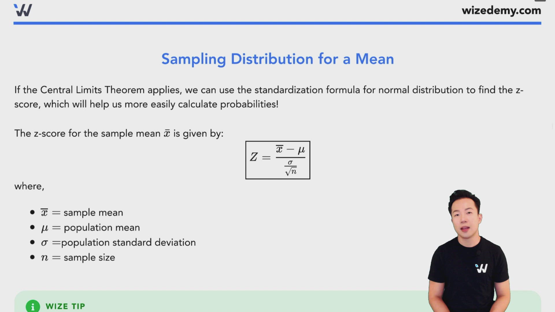
This relationship is governed by the Central Limit Theorem, which states that regardless of the shape of the population distribution, the sampling distribution of the mean will approach a normal distribution as the sample size increases. It’s like magic, but with math!
Key Takeaways About X-Bar and Mu
Here are a few key points to keep in mind:
- X-bar is an unbiased estimator of Mu, meaning it doesn’t systematically overestimate or underestimate the population mean.
- The larger the sample size, the more accurate the estimate of Mu becomes.
- This relationship holds true even if the population distribution is skewed or non-normal.
Understanding this relationship is crucial for anyone working with data, as it forms the basis of many statistical analyses.
How Sampling Distribution Works in Real Life
Let’s bring this concept down to earth with a real-life example. Imagine you’re a coffee shop owner trying to figure out the average amount of coffee consumed by your customers. You can’t possibly measure every single cup sold, so you take random samples of, say, 50 customers each day for a week.
By calculating the mean amount of coffee consumed in each sample and plotting those means, you’ll get a sampling distribution. And guess what? The mean of this distribution will be a pretty good estimate of the true population mean (Mu). Cool, huh?
Applications in Business and Research
Sampling distribution isn’t just for coffee shop owners. It’s used in a wide range of fields:
- Healthcare: Researchers use it to estimate the average effect of a treatment in a population.
- Marketing: Businesses use it to analyze customer preferences and behaviors.
- Education: Educators use it to assess the performance of students in a particular subject.
No matter the field, the principles remain the same: take a sample, calculate the mean, and use it to make informed decisions.
The Central Limit Theorem: The Backbone of Sampling Distribution
Now, let’s talk about the Central Limit Theorem (CLT). This theorem is the reason why sampling distribution is so powerful. It states that as the sample size increases, the sampling distribution of the mean will approach a normal distribution, regardless of the shape of the population distribution.
Here’s why this matters: even if your population data is all over the place—skewed, bimodal, or whatever—once you start taking large enough samples, the means of those samples will form a nice, predictable normal distribution. It’s like chaos transforming into order.
Key Assumptions of the Central Limit Theorem
While the CLT is a powerful tool, it does come with a few assumptions:
- The samples must be independent of each other.
- The sample size should be large enough (usually n ≥ 30).
- The population must have a finite variance.
As long as these assumptions are met, you can rely on the CLT to give you accurate results.
Calculating Sampling Distribution: Step by Step
Now that we’ve covered the theory, let’s get practical. How do you actually calculate a sampling distribution? Here’s a step-by-step guide:
- Take multiple random samples of the same size from the population.
- Calculate the mean for each sample.
- Plot the means on a graph to form the sampling distribution.
- Calculate the mean and standard deviation of the sampling distribution.
And voila! You’ve got yourself a sampling distribution. Easy peasy, right?
Tools and Software for Calculation
While you can do all this by hand, there are plenty of tools and software that can make your life easier:
- Excel: Great for small datasets.
- R and Python: Perfect for larger datasets and more complex analyses.
- Statistical Software: Programs like SPSS and SAS offer advanced features for sampling distribution analysis.
No matter which tool you choose, the principles remain the same: sample, calculate, and analyze.
Common Misconceptions About Sampling Distribution
Before we move on, let’s clear up a few common misconceptions:
- Misconception 1: Sampling distribution is the same as population distribution. Nope! Sampling distribution is about the means of samples, not the individual data points.
- Misconception 2: Larger sample sizes always lead to better results. While larger samples generally give more accurate estimates, they also require more resources.
- Misconception 3: The Central Limit Theorem only applies to normal distributions. False! It applies to any population distribution as long as the sample size is large enough.
Understanding these misconceptions will help you avoid pitfalls in your statistical analyses.
Advanced Topics in Sampling Distribution
For those of you who want to take your stats game to the next level, here are a few advanced topics to explore:
- Bootstrap Sampling: A resampling technique that can be used to estimate the sampling distribution without making assumptions about the population.
- Non-Parametric Methods: Techniques that don’t rely on the assumption of normality.
- Bayesian Statistics: A different approach to statistical inference that incorporates prior knowledge into the analysis.
These topics can take your understanding of sampling distribution to new heights, but they’re also more complex. Start with the basics and work your way up!
Resources for Further Learning
If you’re hungry for more, here are a few resources to check out:
- Books: "Introduction to Probability and Statistics" by William Mendenhall.
- Online Courses: Coursera and edX offer excellent courses on statistics and sampling distribution.
- Websites: Stat Trek and Khan Academy provide free resources for learning statistics.
With these resources, you’ll be a stats pro in no time!
Conclusion: Why Sampling Distribution Matters
Alright, stats lovers, let’s wrap this up. Sampling distribution is not just a dry, academic concept—it’s a powerful tool that helps us make sense of the world. By understanding the relationship between X-bar and Mu, we can draw meaningful conclusions from data without having to analyze every single data point.
So, whether you’re a researcher, a business analyst, or just someone trying to make sense of the numbers around you, sampling distribution is your trusty sidekick. And remember, the Central Limit Theorem is your magic wand, turning chaos into order.
Now, it’s your turn! Leave a comment below and let me know what you think. Are you a stats pro, or are you still wrapping your head around this concept? Either way, I’d love to hear from you. And don’t forget to share this article with your stats-loving friends!
Table of Contents
- What Exactly is Sampling Distribution?
- The Relationship Between X-Bar and Mu
- How Sampling Distribution Works in Real Life
- The Central Limit Theorem: The Backbone of Sampling Distribution
- Calculating Sampling Distribution: Step by Step
- Common Misconceptions About Sampling Distribution
- Advanced Topics in Sampling Distribution
- Conclusion: Why Sampling Distribution Matters
- Finding The Best Flixhdcc Alternatives Your Ultimate Guide
- Unleashing The Power Of Www3 6 Movies Your Ultimate Guide To Streaming Bliss
The Sampling Distribution Of The Sample Mean
All about the sampling distribution of the sample mean — Krista King

SOLUTION Module4 samplingdistributionmean f2021 class Studypool
